

pyZwx User Guide
User Guide of pyZwx
pyZwx User Guide
- 0. Install and Bootup
- 1. Usage flow of pyZwx
- 2. Main Window
- 3. Import an Impedance Spectrum Data
- 4. Z-HIT function (Kramers-Kronig Transformation Test)
- 5. Equivalent Circuit Editor and Circuit Script
- 6. GUI Support Function to Find a Good Initial Guess
- 7. Least Sqared Fitting
- 8. Data Mask
- 9. Numeical Data Table
- 10. Simulation
- 11. Save Window Layout
- 12. Misc
0. Install and Bootup
pyZwx is Windows version only.
Download zipped pyZwx 64 bit or 32 bit version and save in your computer. pyZwx can be used by unzip that file.
You can save pyZwx in any folder you want.
pyZwx boots up by doule clicking pyZwx64.exe or pyZwx32.exe.
Attention:For bootup of pyZwx, about 15 seconds are necessary. Please wait until open a main window.
Return to the top.1. Usage flow of pyZwx
Analysis flow by pyZwx is:
- Load a impedance spectrum data
- (Check the spectrum by Z-HIT test)
- Input an equivalent circuit model and its initial guess values
- Run a complex nonlinear least squares
- Save the fitted results
2. Main Window
Main frame containing main menu appears at an initial bootup.
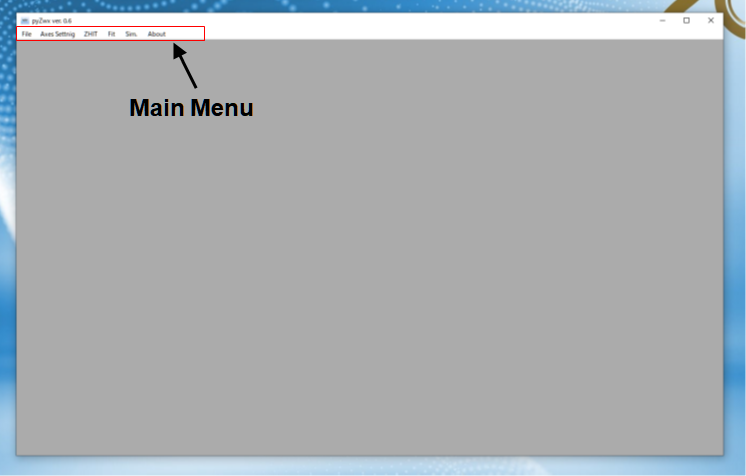
Items of the main menu are the followings:
- File
- Menu for import file selection.
- Axis Setting
- Setting of the maximum and minimum values of displayed plots. Regarding to an impedance plot, this setting is not worked because of an automatic setting that axis aspect is automatically equal.
- ZHIT
- Operation of Z-HIT test.
- fit
- Call an Equivalent Circuit Editor.
- Sim.
- Call Simulation Setting Editor.
- About
- About a license and link to this web site.
3. Import an Impedance Spectrum Data
Spectrum data file can be imported by "Load Data File" in "File" menu. User can select a file on a file dialog. Following formatting files can be imported without modification.
- z (ZView, Scribner)
- There is possibility to fail importing when a *.z file is generated by a software released by other than Scribner.
- mpt (EC-Lab, BioLogic)
- Regarding to a *.mpt file including multiple spectra data, pyZwx can't import all the data. For such file, you can split each spectrum data by "Split Mpt File" command in File menu. When mpt file is failed to import, please try to split spectrum data using Split Mpt File command.
- Extension name of convert ZView format data by EC-Lab becomes "txt". This file can be imported without modification.
- par (Versa Studio, Princeton Analytical Research)
- *.par file can be imported without modification. Do not convert ZView format by Versa Studio.
- dta(Gamry Framework, Gamry)
- *.dta file output by Gamry Framework ver. 6.3 was confirmed to be importable.
- idf (IviumSoft, Ivium Technologies)
- *.idf file output by IviumSoft ver. 4.9 was confirmed to be importable.
- txt
- Useful delimiters: tab, space, comma. These are automatically identified.
- No headder or one line text hedder for each columns are permitted.
- Data array: frequency, $Z_{\text{real}}$, $Z_{\text{imag}}$. Do not change sign of $Z_{\text{imag}}$.
- SMaRT (Scribner) output file
- Regarding to *.dat file output by SMaRT software (Scribner Associates), exported csv file can be loaded by following procedures by SMaRT.
- Check "Status grid and table/CSV quantitiles" term displayed by "Tools" menu => "Options.." submenu => "Experimence" tab.
- "1" is set at "Impedance" and "Real", and "2" is at "Impedance" and "Imaginary".
- Csv format text is exported by "Export Data File" submenu.
- The extension name is changed from txt or csv to smt.
- fit (pyZwx)
- *.fit file saved by pyZwx can import. This file can be made at "File" menu of Equivalent circuit editor.
- Top: Full file name including file path name.
- Right side: logarithm of frequency versus (top) real part of impedance (Zreal), (middle) logarithm of absolute Zreal, and (bottom) residual between measured data and calculated one (delta Zreal).
- Center: logarithm of frequency versus (top) imaginary part of impedance (Zimag), (middle) logarithm of absolute Zimag, and (bottom) residual between measured data and calculated one (delta Zimag).
- Left side: Impedance (top) and interactive 3D plots.
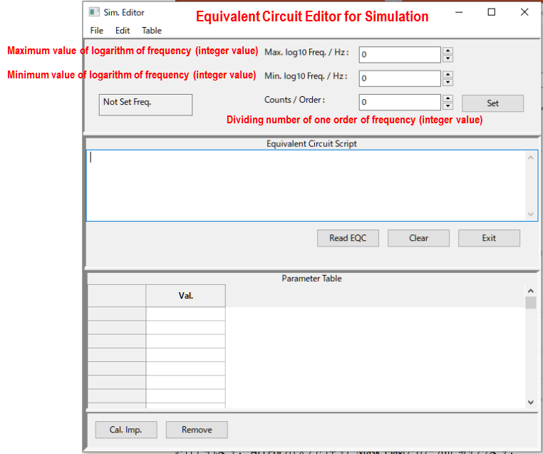
- Maximum and minimum values of logarithm of frequency must input by interger number.
- Dividing number per one order of frequency must input by integer number. The division is made by equal space in logarithmic scale.
- Frequency will generated when you push "Set" button. If frequency array is successfully generated, ”Success to Generate the Frequency!" popup will be displayed.
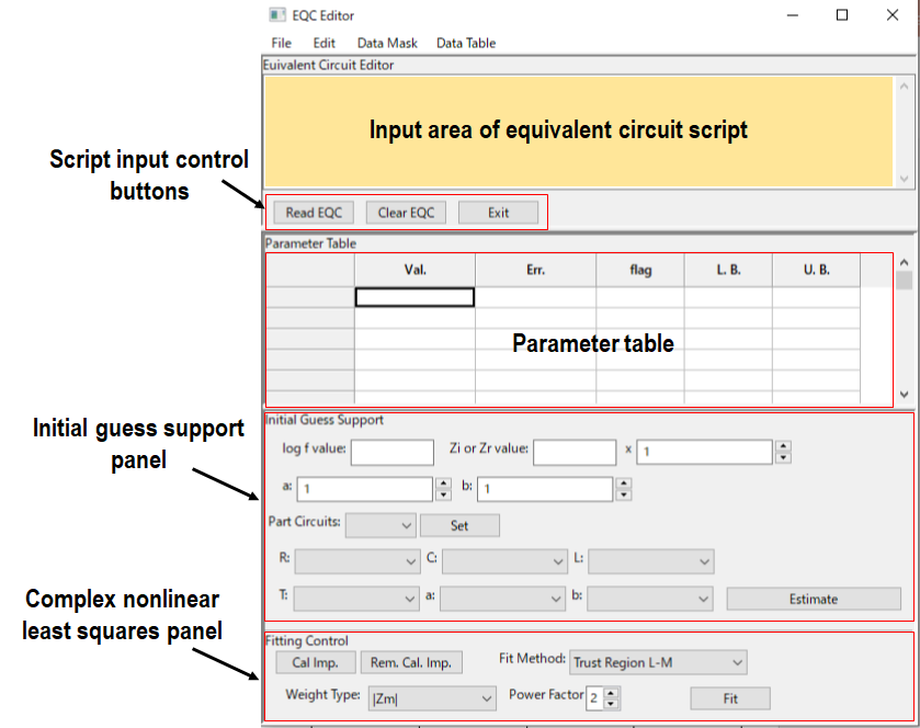
- Type an equivalent circuit script and push "Read EQC" button, parameter table is displayed. After input parameter values, you can make simulated spectrum by pushing "Cal. Imp" button. Simulated spectrum is displayed on main window.
- Data table is displayed when you select "Show Table" submenu in "Table" menu at simulation editor window. This table is also possible to copy to clipbord by druggin and select "Copy" submenu in "Edit" menu at simulation editor window. In addition, this cpied data is also possible to paste on other softwares.
Split Mpt File submenu
User can split each spectrum data file from a *.mpt file including multiple impedance data. The names of splitted files are "[original file name]#[2 ordered number].txt".
If a file is successfully imported, file name including full path name, eight plots, navigation toolbar for GUI operation of the plots are displayed in the main window.
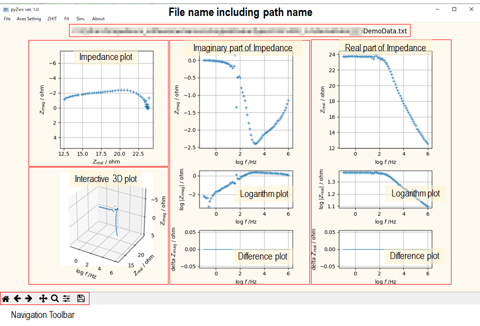
Displayed plots after data import are followings:
Navigation toolbar is displayed after data import. This tool bar is used for GUI operations of displayed graphs.
The tool bar was implemented using the function of Matplotlib module. About the tool bar, please refer to "Matplotlib vre. 3.1.2 documentaion".
 Return to an initial state button.
 Back state button.
 Forward state button.
 Pan/Zoom button. After pushing this button and move a mouse cursor inside of a graph. Then, mouse is moved with keeping pushing left button,
you can move a graph plot inside that region. If you move the mouse with pushing right button, the plot expands or shrink according to the mouse movement.
Pan/Zoom button. After pushing this button and move a mouse cursor inside of a graph. Then, mouse is moved with keeping pushing left button,
you can move a graph plot inside that region. If you move the mouse with pushing right button, the plot expands or shrink according to the mouse movement.
 Zoom to recutangle button. After push of this button and move a mouse cursor inside of one graph. You can select a zoom up region by dragging the mouse with
 Sub-plot configulation button. You can tune spaces between the graphs.
 Save image button. You can save an image of main window only.
Interactive 3D plot can be rotated by mouse operation, other function by Navigation toolbar cannot be used.
Return to the top.4. Z-HIT funcction (KK Transformation Test)
Z-HIT is Hilbert Intergral Transformation test of impedance (Z) spectrum.Kramers - Kronig transformation test is a checking method that an impedance spectrum can be solved by an equivalent circuit model. By conventional KK transformation test is applicable to a spectrum that the imaginary part is close to 0 at high- and low-frequency limits. Therefore, conventional KK transformation test can not be used for spectra collected by batteries, capacitors, and so on.
Z-HIT is a transformation test based on different empirical equation reported by Ehm at 2000.
W. Ehm, H. Gohr, R. Kaus, B. Roseler, C. A. Schiller, "The evaluation of electrochemical impedance spectra using a modified logarithmic Hilbert transform", ACH Models in Chem. 137 (2000) 145-157. DOI:10.1039/b007678n
Z-HIT is applicable to impedance spectra of batteries and capacitors.Usage of Z-HIT
After loading data, Z-HIT result will be displayed by selecting "do ZHIT" submenu at "ZHIT" menu. If a measured spectrum show good agreement with Z-HIT results, this indicates that the measured spectrum can be reproduced by an equivalent circuit model. Inversely, a measured spectrum is different from Z-HIT result, the spectrum is difficult to reproduce by an equivalent circuit model.
Impedance spectrum collected using a coin-type lithium battery (CR1620) is shown as an example. In the case of this spectrum, measured spectrum and Z-HIT result show large difference below 0.1 Hz. In addition, the difference becomes larger with decreasing freaquency. Therefore, this measured spectrum can be solved by an equivalent circuit model only higher than 0.1 Hz.
Causes to collect an impedance spectrum which cannot be solved by an equivalent circuit is lack of causality, linearity, and stability. As you see, you can obtain preinformation about spectrum analysis by Z-HIT.
Attention: It has been confirmed that Z-HIT cannot well evaluate spectrum including resistor connected to inductor parallelly. So, you need to pay attention about this point.
You can save the Z-HIT results by selecting "Save Result" submenu in "ZHIT"menu.
You can remove the Z-HIT curve on the main window by selecting "rem. ZHIT" submenu.
5. Equivalent Circuit Editor and Circuit Script
After loading data, you can open Equivalent Circuit Editor window by selecting "Equiv. Cir. Editor" submenu in "Fit" menu.
Equivalent circuit is described by peculiar script. Circuit elements, their parameters, equations, and label index are listed in below table.
ω:Angular frequency = 2πf.f:frequency.j:imaginary unit.
| Element Name | Index | Equation (Z = ) | Parameter | Label |
|---|---|---|---|---|
| Resistor | R | $R$ | R | R01, R1, R001, etc |
| Capacitor | C | $\frac{1}{(Cjω)}$ | C | C01, C1, C001, etc |
| Inductor | L | $Ljω$ | L | L01, L1, L001, etc |
| Constant Phase Element | CPE | $\frac{1}{T(jω)^α}$ | T, α | CPE01, CPE1, CPE001, etc |
| Infinite diffusion length Warburg Impedance | W_old | $\frac{1}{T(jω)^α}$ $α $= 0.5 is ideal |
R, T, α | W_old01, W_old1, W_old001, etc |
| Finite diffusion length with transmissive boundary Warburg Impedance | W_fc | $[\frac{R}{T(jω)^α}]\text{tanh}\{T(jω)^α\}$ $α $ = 0.5 is ideal |
R, T, α | W_fc01, W_fc1, W_fc001, etc |
| Finite diffusion length with reflective boundary Warburg Impedance | W_sb | $[\frac{R}{T(jω)^α}]\text{coth}\{T(jω)^α\}$ $α $ = 0.5 is ideal |
R, T, α | W_sb01, W_sb1, W_sb001, etc |
| Gerischer Impedance | G | $\frac{R}{\{T+(jω)^α\}^β}$ $α$ = 1 and $β$ = 0.5 are the ideal |
T | G01, G1, G001, etc |
| Havliriak-Negami Impedance | HN | $\frac{R}{\{1+(Tjω)^α\}^β}$ | T | HNG01, HN1, HN001, etc |
| Serial Connector | + | NA | NA | NA |
| Parallel Connector | // or / | NA | NA | NA |
| Block | (), {}, and [] | NA | NA | NA |
This script rule is the same with the following reference.
K. Kobayashi, T. S. Suzuki, Electrochem., 88 (2020) 39-44. DOI:10.5796/electrochemistry.19-00058
About theoretical aspects of Warburg impedances and Gerisher impedance, please see the following reference.
K. Kobayashi et al., Solid State Ionics, 249-250 (2013) 78-85. DOI: 10.1016/j.ssi.2013.07.022
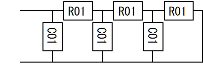
Followings are the examples of equivalent circuit script. The graphical circuit,
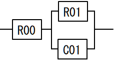
Approximated circuit to express Warburg impedance is graphically presented by,
Non zero values should input at the Val. column before pushing "Cal Imp." and "Fit" button.
After typing equivalent circuit script and push "Read EQC" button, input table is displayed in the parameter table area. As an example, parameter table
generated using the script "R01+R02//C02" is shown in below figure.
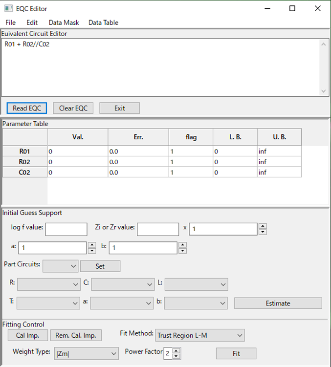
Meanings of the column are the following:
Val.column: Parameter input
Err.column: Standard uncertainty output by complex nonlinear least squares
flag column: Parameter flag.1: variable; 0: fix
L. B. column: Lower bound of corresponding parameter. If you want to set at nonconstrain, please input -inf instead of 0
U. B. column: Upper bound of corresponding parameter
Upper and lower bounds of power law factor (α, β) are automatically set at 0 and 1, respectively. If you want to change this setting,
please input different values at L. B and U. B columns.
Regarding to Warburg and Gerischer impedances, power law factor value is set at ideal value with fixed condition (flag = 0).
If you need to change this setting, please change the flag setting.
In the case of Demo_data.txt in the Demo data folder, you can solve by following models and initial guesses. Parameter values can input in the table cell manually.
Model 1
R0 + R1//CPE1 + R2//CPE2 + R3//CPE3
R0: 11
R1: 3; CPE1_T: 1e-6; CPE1_a: 0.9
R2: 3; CPE2_T: 1e-4; CPE2_a: 0.9
R2: 3; CPE2_T: 1e-2; CPE2_a: 0.9
Model 2
R0 + R1//C1 + R2//C2 + R3//C3 + R4//C4 + R5//C5 + R6//C6
R0: 12
R1: 3; C1: 1e-7
R2: 2; C2: 5e-6
R3: 2; C3: 1e-6
R4: 2; C4: 5e-5
R5: 2; C5: 1e-5
R6: 2; C6: 5e-4
6. GUI Support Function to Find a Good Initial Guess
This is a new function of pyZwx ver. 1.0. Good initial guess can set by GUI operation; selection of partial impedance model and sampling data. Initial guess support panel is located at the middle of the equivalent circuit editor. Setting is made using; partial impedance model popup; its setting button; parameter selection popups; estimate button.
You can find the equations used for this function by;
K. Kobayashi, T. S. Suzuki, Electrochem., 88 (2020) 39-44. (Open Access) DOI:10.5796/electrochemistry.19-00058
As an example, usage procedures are explained using DemoData.txt in the demoData folder. After import this data, following plots are displayed in the main window. This spectrum is solved by "R0 + R1//CPE1 + R2//CPE2 + R3//CPE3" model.
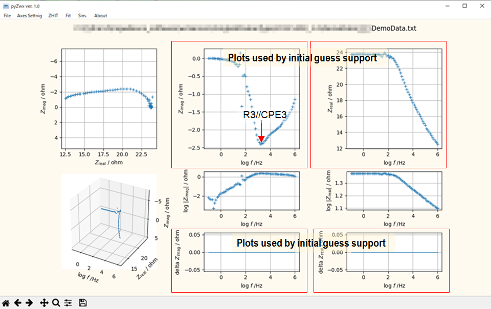
The plots of $\text{log} f - Z_{\text{imag}}$, $\text{log} f - \text{delta }Z_{\text{imag}}$, $\text{log} f - Z_{\text{real}}$, and $\text{log} f - \text{delta }Z_{\text{real}}$ are interactively used for the initial guess support.
Open equiavlent circuit editor, input the script by "R0 + R1//CPE1 + R2//CPE2 + R3//CPE3", and then push the "Read EQC" button. By these procedures, parameter table is displayed. Then, the point shown at the red arrow in the above figure is clicked. Text controls of "log f value" and "Zi or Zr value" in the initial guess support panel are automatically filled values. These are picked up ones by the click on the plot.
Next, R3//CPE3 element is pushed with peak at the clicked position. Select a "R//CPE" from the "Part Circuit" popup in the initial guess support panel and then, push the "Set" button localted at rightside of the popup. By this setting, parameter table list is transfered to each parameter popups. In the case of R//CPE, settable parameters are "R", "T", and "a".
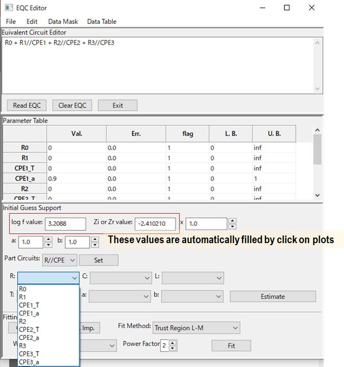
Select "R3", "T3", and "a3" from the "R", "T", and "a" popups in the initial guess support panel, respectively and then, push the "Estimate" button. By this procedure, T3 value is calculated using log f value, Zi value, and a value showin in "a" toggle. The calculated spectrum is displayed on the plots.
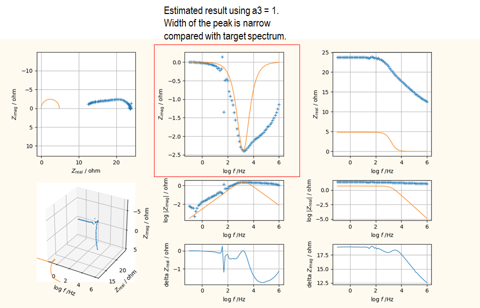
Estimated spectrum is found to be narrow peak compared with target spectrum. The reason is that model spectrum is calculated with a3 = 1 that is set at "a" toggle just below the "log f value" label. The width of the peak can be expanded by setting at smaller than 1. Change the "a" toggle value from 1 to 0.8 and then, push the "Estimate" button, the calculated spectrum is changed to be closed to the target spectrum.
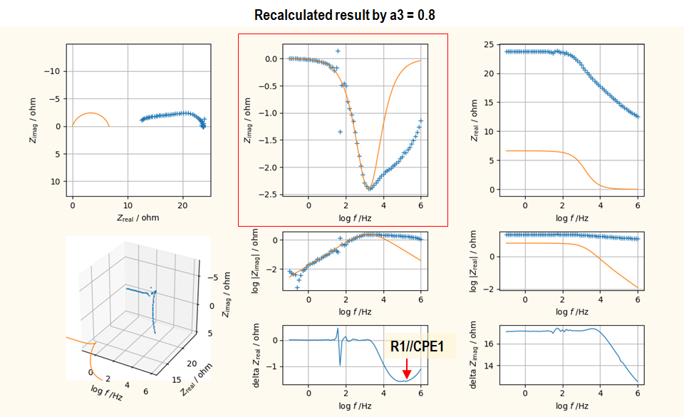
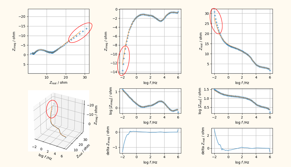
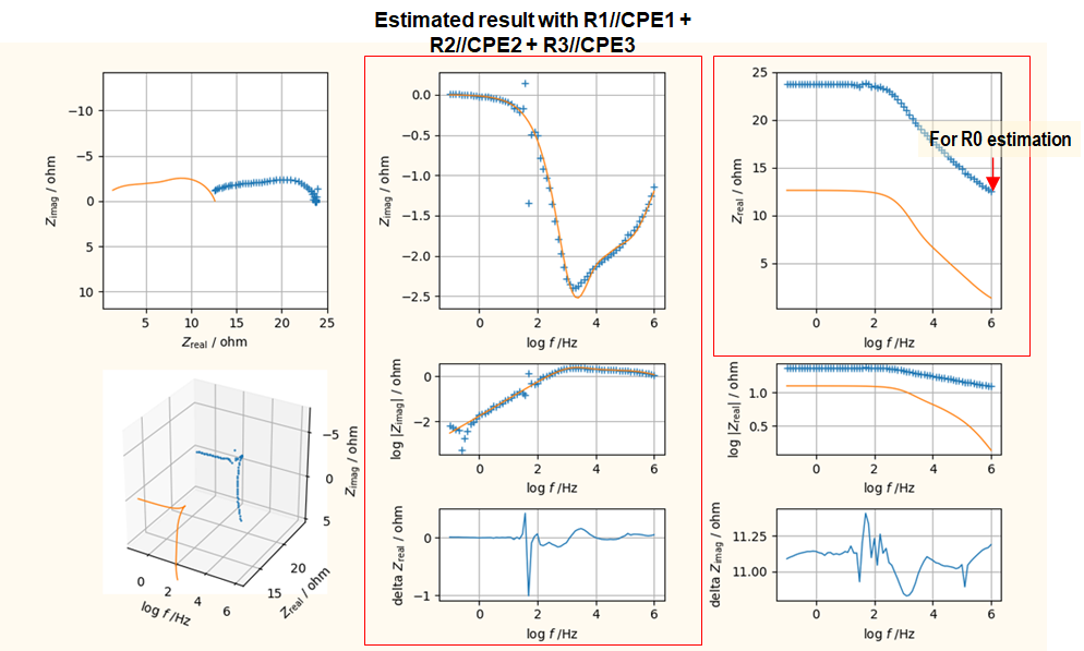
At this stage, $\text{log} f - \text{delta} Z_{\text{imag}}$ curve becomes a substracted one by R3//CPE3 element. Therefore, the residual R1//CPE1 and R2//CPE2 element informations are also left in this curve. Next, the point shown by the red arrow in the above figure is clicked. At this case, "log f value" and "Zi or Zr value" are filled at the residual curve data. Then, set the "a" toggle at 1, select "R1", "T1", and "a1" from the "R", "T", and "a" popups, respectively. By pushing "Estimate" button, calculated spectrum is refleshed in the plots. By this results, peak shape of R1//CPE1 is also found to be narrow as similar to the R3//CPE3, peak is expanded by changing a from 1 to 0.6 and then, push the "Estimate" button. The result is shown in the below figure.
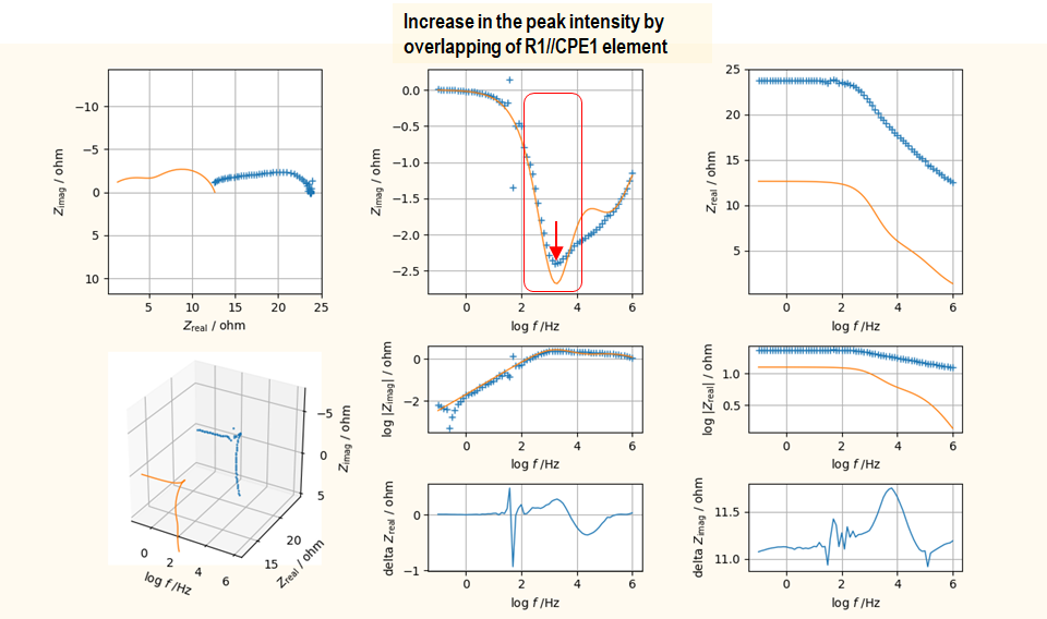
Peak intensity at R3//CPE3 becomes strong because of overlapping of R1//CPE1 element. So, it is necessary to tune the R3//CPE3 parameter. Click at the point shown by red arrow in the above figure, "a" toggle value is set at 0.8, and then, push the "Estimate" button. Next, proportional factor shown in the below figure is set at 0.9 (smaller than 1), and then push "Estimate" button. You woould see that peak by R3//CPE3 is weaken. If the peak intensity is too small, it is possible to increase that by setting the proportional factor at 1.1 (larger than 1) and then, push "Estimate" button.
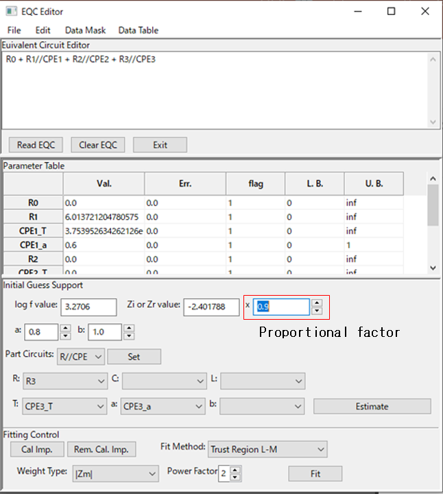
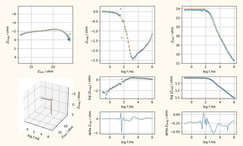
At this state, you may find that R//CPE element with the peak at log f is close to 4.5 from the $\text{log} f - \text{delta} Z_{\text{imag}}$ curve. If you push R2//CPE2 element at this region, the estimated spectrum is like following figure. This is not the optimizing procedure but the estimate of initial guess for complex nonlinear least squares. Therefore, small deviation is amost no problem. At last, the point shown by red arrow in following figure is clicked in order to estimate "R0". Then, "R" is selected in the "Part Circuits" popup and push the "Set" button. Then, select "R0" from "R" parameter select popup and push "Estimate" button. For R0 tuning, proportional factor can be used.
Finally, good initial guess can be set by GUI operation only.
Manual input of "log f value" and "Zi or Zr value" are possible.When a frequency at peak position is out of measured frequency region, estimated peak frequency and Zi ro Zr values input manually and then, are tuned using proportional factor.
Return to the top.7. Least Sqared Fitting
Complex nonlinear least squares starts when you push "Fit" button. When the calculation converges, output log from LMFIT library and comment input window will be displayed. Then, values of Val. and Err. columns in the parameter table are changed from the initial guess to the optimized ones. Regarding to statistic values in output log by lmfit, please check LMFIT home page.
Comment input in the comment input window is saved in *.fit file when you save your fitted results by selecting "Save Fitted Results.." submenu in "File" menu on Equivalent Circuit Editor window.
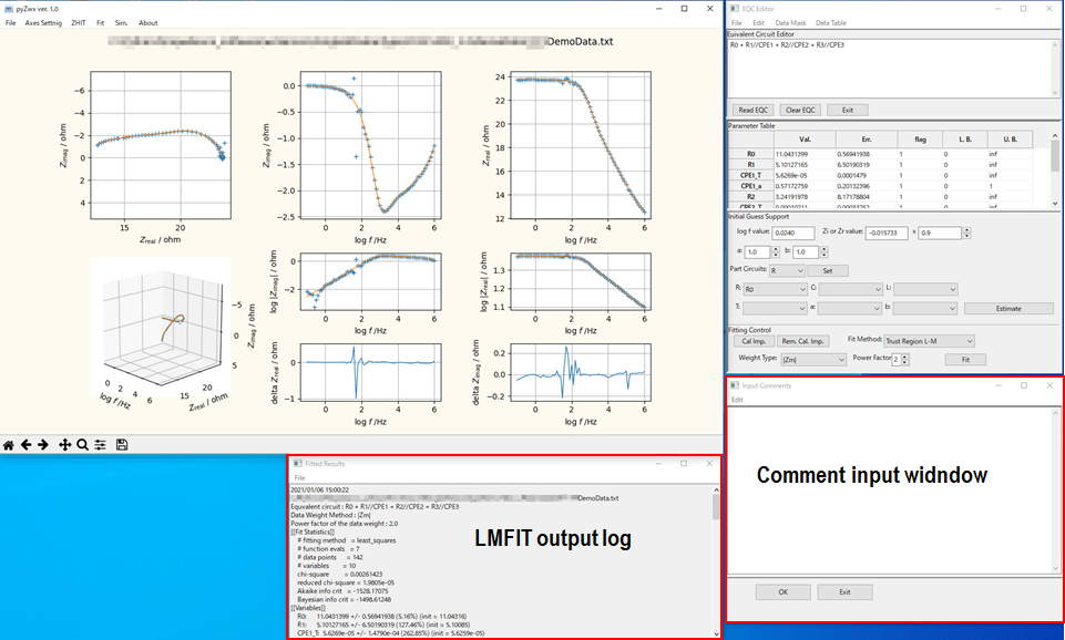
Usually fitting is finished within one minit. If Lmfit log window and Memo input window do not appear after pushing "Fit" buttons, it may be a result by fail of calculation. This error can be prohibit by use of initial guess support.
From "Fit Method" popup in the fitting control panel, nine algorithm for complex nonlinear least squares are selectable. Trust-region Lebenberg-Marquardt method is the default algorithm. Depending on the optimizing algorithm, calculation of a standard uncertainty is failed and as the result, error occurrs. Within my test, trust-region Lebenberg-Marquardt algorithm is most stable for impedance analysis.
If you want to fit by "Modulus weight" and completely the same with other impedance analysis softwares, set "|Zm|" or "|Zcal|" of Weight Type and set at 2 of the power factor in the Equivalent circuit editor window.
If you do not use data weight, select "Unit Weight". In the case of unit weight, power factor has no influence.
If you want to fit by "Proportional weight" and completely the same with other impedance analysis softwares, set "|Zm_r| & |Zm_i|" or "|Zcal_r| & |Zcal_i|" of Weight Type and set at 2 of the power factor in the Equivalent circuit editor window.
After drugging the parameter table region and select "Copy" submenu in "Edit" of equivalent circuit editor window, table values are copied to clipbord.You can paste that data to other softwares such as excell etc.
Attention: Short cut key is NOT working to the table copy.
If you save your fitted results by "Save All of Fitted Results as" submenu in "File" menu of equivalent circuit editor, equivalent circuit model, comments you input, parameter names, optimized values, their uncertainties, output log by Lmfit, measured spectrumd data, model spectrum data, masked data are saved in one file. The extention name is "fit". This file is text format with UTF-8 encode. So, you can open the file using text editor.
Return to the top.8. Data Mask
pyZwx has a function to mask some data that are not used for complex nonlinear least squares. Masked data DO NOT disapper but change color.This function is effective when you know that a part of data cannot be fit by a model due to the Z-HIT results and clarly deconvolute large noise.
When you use the mask function, its control window is displayed by selecting "Data Mask" submenu at "Data Mask" menu of equivalent circuit editor.
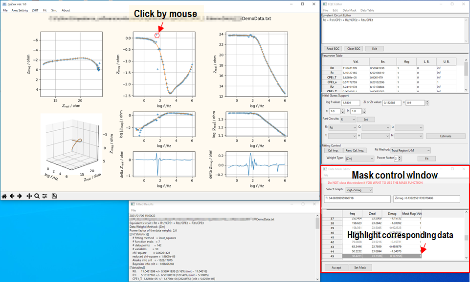
Mask control window is opened. If you click on log f - Zimag plot close to one marker that is a data you want to mask, corresponding data is highlighted in the mask control window. If you push "Accept" button, corresponding flag cell value is changed from 1 to 0. When you push "Set Mask" button, the data is masked and the color of the marker is changed to green.
Mask setting can be done by manual input at 0 of flag cells.
Attention: DO NOT close the mask control window if you want to use the mask function. Mask setting information disappears when the mask control window is closed.
Return to the top.9. Numeical Data Table
Numerical data table is displayed when you select "Data Table" submenu in "Show Data Table" menu on equivalent circuit editor window. On this table, measured spectrum, model spectrum, difference between measured data and calculated one, and so on are contained. This table can be copied on clipbord by selecting of "Copy" sbmenu in "Edit" menu on equivalent circuit editor window. This copied data can paste on other softwares such as excell.
Return to the top of this Page.10. Simulation
Simulation control window can be opened by selecting "Sim. Eqc. Editor" submenu in "Sim." menu on main window.
You can simulate a spectrum using this control window.
11. Save Window Layout
You can save windows layout of pyZwx. Adjust window layout by mouse operation and then, you can save that by Setting menu => Save Present Appearance. When you save the layout, pyZwx.ini file is formed at the same folder locating pyZwx.exe. If you want to clear the layout, you can delete that by Setting menu => Reset Default. Or the layout is reset if you delete the pyZ.ini file.
Return to the top.12. Misc
If pyZwx is not working well by some operation, please close main window and reboot that.
Return to the top.