

Basics of analysis
- 1. Basics of impedance
- 2. Example of capacitor impedance
- 3. Meaning of emprical parameters (Example of Debye's empirical spectrum)
- 4. Complex nonlinear least squares
- 5. Data weighting method implemented in pyZwx
- 6. Equivalent circuit
- 7. Data structure of impedance and its display method by graphs
- 8. Impedance and complex permittivity
1.Basics of impedance
"Impedace" is a coined word by O. Heaviside (1850-1925). That origin of the word is "impede" which has means "hinder or obstruct the progress or movement." Difference between impedance and resistance is that impedance was defined in a world of wave signals. The world of wave signals is the same with Fourier domain on the basis of present knowledge. Relationships between impedance, time domain, Laplace domain, Fourier domain were compactly explained in the review by D. D. Macdonald. Impedance was born as one concept to explain the reason that transmitted signals was changed from the initial signal during long journey in transatlantic telegraph cable at Victorian age. Note that oscilloscope had not been developed yet at that time. He understood that change only from initial electromagnetic theory. Response signal is different from the input signal indicate that response signal should be represented at least by linear differential and/or integral equations.
Briefly review Laplace transform, Heaviside transform, and Fourier transform. (Ex. Wiki page)
It is assumed that a function of time, $f(t)$, is satisfied with $f(t) = 0$ at $t < 0$ and $\int_{-\infty}^{\infty}|f(t)|dt < \infty$ is given by,
$F(s) = \int_{0}^{\infty}f(t)e^{-st}dt \ \ \ \ \ $(1-1)
where $s$ is Laplace variable and given by complex number, $s = \sigma + j\omega$. $\sigma$ represents a real part of s. On the other hand, $\omega$ represents angular frequency on the basis of Euler's formula.
Equation (1-1) represents that Laplace transform is mathematical mapping from function of time, f(t), to function of complex number, s. In order to simplify an expression, Laplace transform is represented by the following form.
$F(s) = \mathcal{L}[f(t)] \ \ \ \ \ $(1-2)
Combined with derivative and integral of composite functions, following relationships can be derived.
$\mathcal{L}[\frac{df(t)}{dt}] = sF(s) - f(0)\ \ \ \ \ $(1-3)
$f(0)$ is an initial value. Response signal of impedane measurement is independent of $f(0)$ and therefore, $f(0)$ is equal to 0. From equations (1-3) and (1-4), it is found that linear derivative and/or derivative operator is removed by Laplace transform and as the results, the transformed equation becomes simple forms. New domain mapped by Laplace transformation is called by "Laplace domain".
Heaviside transform is a mapping from Laplace domain to Fourier domain by replacement of $s$ to $j\omega$. A reason why direct transformation from a function in time domain to Fourier domain does not conducted is that there are cases that Fourier transformation equation corresponding to (1-1) diverges or is equal to 0. In these cases, it is impossible to define an impedance. In the case of electrochemical impedance, it is not necessary to derive concrete functions of $f(t)$ and $F(s)$. It is enough to understand that functions of current and voltage in time domain are transformed by current and voltage as functions of different variable, $s$, and $j\omega$.
After mapping of current[$i(t)$] and voltage [$v(t)$] functions in time domain to Fourier domain [$I(j\omega)$ and $V(j\omega)$] by Laplace transform and subsequent Heaviside transform, impedance [$Z(j\omega)$] is derived by $I(j\omega)/V(j\omega)$ as similar to Ohm's law. It is possible to understand that impedance is a function of $j\omega$ not $\omega$.
Sometimes, we find an explanation like that "a.c field is applied, voltage and current is proportional to $e^{j\omega t}$...". This method is a simple alternative of Laplace transformation and subsequent Heaviside transformation. But it is a problem that there is no explanation of a concept of "transformation." Because such explanation is ambiguous which domain he explained. Explanation like following is so ambiguous: "Actual time domain, real part of the $V_{0}e^{j\omega t}$ is the applied voltage, and real part of $I_{0}e^{j\omega t}$ is measured as the current." It is natural feeling that curious explanation is curious.
Return to the Top2. Example of capacitor impedance
It is assumed that capacitor ($C$) is represented by derivative form, and relationship between electric charge ($Q$) and voltage ($v$) is given by,
$C = \frac{dQ}{dv} \ \ \ \ \ $(2-1)
If $Q$ and $v$ are functions of time, following equation can be derived by derivative with respect to time,
$\frac{dQ(t)}{dt} ≡ i(t) = C\frac{dv(t)}{dt}\ \ \ \ \ $(2-2)
By applying equation (1-3) and Heaviside transformation to (2-2), function at Fourier domain is derived,
$I(j\omega) = Cj\omega V(j\omega)\ \ \ \ \ $(2-3)
Impedance can be derived by its definition,
$Z(j\omega) = \frac{V(j\omega)}{I(j\omega)}= \frac{1}{Cj\omega}\ \ \ \ \ $(2-4)
You may understand that v/i is difficult to derive from equation (2-1) but it is easy from equation (2-3).
Return to the Top3. Meaning of empirical parameters (Example of Debye's empirical spectrum)
Inversely derive the time domain equation of Debye's empirical spectrum (R//CPE) in Fourier domain. Because physical and/or mathematical mean of CPE parameters become clear.
Impedance equation of R//CPE is presented by,
$Z(j\omega) = \frac{V(j\omega)}{I(j\omega)} = \frac{R}{1+RT(j\omega)^{\alpha}}\ \ \ \ \ $(3-1)
$R$ is resistance, $T$ is a pseudo capacitance of constant phase element (CPE), $\alpha$ is called a parameter to present dgree of decompress of circule, fractal parameter, etc. Reciprocal to equation (3-1), you can derived the following equation,
$I(j\omega) = \frac{V(j\omega)}{R} + T(j\omega)^{\alpha}V(j\omega)\ \ \ \ \ $(3-2)
Note that equation (3-2) cannot be transformed by (1-3), because it is impossible to explain the $(j\omega)^{\alpha}$ term. Remind that $j\omega$ term was generated by (1-3) and subsequent Heaviside transformation due to derivative with respect to time. If similar rule exists, it is possible to speculate that $(j\omega)^{\alpha}$ would appear by $\alpha$-th derivative with respect to time. Non-integer number of derivative exists in mathematical field of "fractional calculus." (Monograph 1,Monograph 2) Referring to this mathematics, equation (3-2) can be transformed as following,
$i(t) = \frac{v(t)}{R}+ T\frac{d^{\alpha}v(t)}{dt^{\alpha}}\ \ \ \ \ $(3-3)
$\frac{d^{\alpha}}{dt^{\alpha}}$ is a fractional derivative operator with respect to time. Pseudo capacitance, $T$ is a coefficient of fractional derivative of $v(t)$ with respect to time. α$\alpha$ is the order of the derivative. By impedance analysis, order of derivative is parameterized! In addition, unit of $T$ includes $\alpha$. The $\alpha$ is vanished only when the $\alpha$ is equal to 1.
Fractional calculus is constructed to complement of integer-number of calculus and therefore, physical view scope is ambiguous. Hence, physical scope of (3-3) is also quite ambiguous. As the results, followings are concluded.
- There is no physical scope in R//CPE spectrum model
- No change exist for the definition of resistor
- Pseudo capacitance is completely different parameter from capacitor
- There is no warranty that resistor separated by R//CPE has physical mean
CPE and empirical parameter should not be used. In many cases, we must speculate an equivalent circuit model only by observation of spectrum shape. In such situation, CPE and empirical parameter become necessary evil because we must set a model under insufficient information. It is necessary to know that if you fit a spectrum by empirical Warburg and Gerischer model, it is the same mean that you deny Fick's diffusion laws, particularly the second law. If you use empirical parameters, you must make up you mind that present physical model is denied and must have responsibility to explain the reason and propose new models.
New software exists that non-ideal shaped spectrum can be fit with no use of empirical parameters.
K. Kobayashi, Y. Sakka, "Development of an electrochemical impedance analysis program based on the expanded measurement model", J. Ceram. Soc. Jpn., 124 (2016) 943-949.DOI: 10.2109/jcersj2.16120
K. Kobayashi, T. S. Suzuki, "Development of an Algorithm for Automatic Analysis of the Impedance Spectrum Based on a Measurement Model", J. Phys. Soc. Jpn., 87 (2018) 034004.DOI: 10.7566/JPSJ.87.034004
But this methodology and its importance have not been made consensus.
Retrun to the Top4. Complex nonlinear least squares
At present, impedance is presented by complex function or number. By complex nonlinear least squares, data is fit by complex function under constraints that all parameter is real numbers. This complex nonlinear least squares can be operated by nonlinear least square module implemented at some free programing environments (Ex. Scilab and R). Detail method to write code is depending on programming language and therefore, abstract is explained here. The procedures are the followings:
- Code a function that return a complex impedance value when parameter list and frequency valuese input
- Code a function that checking input frequency list size and if the frequency is localted upper than a half-size, return the real part of the impedance. Oppositely, the frequency is localted lower than a half-size, return the imaginary part of the impedance.
- Frequency list is concatenated. As the result, twice size of the frequency list is made as new list.
- Two lists, measured impedance at real part and imaginary part, are concateneted into one list. This is also made as new list
- Nonlinear least squares are conducted using function (2) and lists (3) and (4)
By the above method, sum of the least squares (S) is presented by following equation:
$S = \sum_{k=0}^{k=l-1}\frac{\left(Z^{data}[k]-Z^{model}_{real}[k]\right)^2}{w[k]} + \sum_{k=l}^{k=2l-1}\frac{\left(Z^{data}[k]-Z^{model}_{imag}[k]\right)^2}{w[k]}\ \ \ \ \ (4-1)$
l is the number of measured data, $Z^{model}[k]$ is the data list explained by procedure (4) above, $Re()$, $Imag()$ are the function to output the real and imaginary part of complex number, $Z^{model}[k]$ is the impedance model function that returns a complex value when freuency list made by procedure (3) is input, $w[k]$ is data weight coefficient of $k$th data. $w[k]$ is ideally given by standard deviation of each data. About the data weight, detail explanation is given at next section.
Return to the Top5. Data weighting method implemented in pyZwx
Usually, standard deviation of each data are not output for impedance measurements. Hence, data weight coefficient is set by values which would be proportional to standard deviation. In addition, standard uncertainty is calculated by normalization by the sum of the least squares. In the case of impedance analysis, $w[k] = |Z[k]| = \sqrt{Z^{2}_{real}[k] + Z^{2}_{imag}[k]}$ is employed in many software. $Z_{real}[k]$ and $Z_{imag}[k]$ are real and imaginary parts of the impedance at $k$th frequency generated at procedure (3). Depending on the weighting method, $Z_{real}[k]$ and $Z_{imag}[k]$ are used for measured data and calculated ones. In the case of pyZwx, measured data is selected if you set "Weight Type" at |Zm|. Insteadly, calculated values are selected when you set that at |Zcal|.
In the case of pyZwx, data weight function is coded by the following form in order to be generalized:
$w[k] = \left(Z^2_{real}[k] + Z^2_{imag}[k]\right)^{pf/4}\ \ \ \ \ (5-1)$
$pf$ is the Power Factor set at the Equivalent Circuit Editor. The reason that the power factor is variable is that optimum power factor seems to be different depending on data and optimizing algorithm.
Note about an implicit assumption of the $w[k] = |Z[k]| = \sqrt{Z^{2}_{real}[k] + Z^{2}_{imag}[k]}$ weight. By this weight, standard deviation of real and imaginary parts of the impedance at fixed frequency are assumed to be the same to each other. If we assume that real and imaginary parts of impedance data have different standard deviations, different setting is necessary. The different setting is that data weight coefficient of the real and imaginary parts are different values. Such setting corresponds to the "|Zm_r| & |Zm_i|" and "|Zcal_r| & |Zcal_i|" of the weight type. By this setting, standard deviation of real and imaginary parts are assumed to be proportional to each values. This assumption is felt to be good, but this method has strong tendency to diverge and therefore, this is not practical one.
No use of data weight is "Unit weight". By this setting, all of the $w[k]$ are set at one. This weight method is valid when the $|Z|$ data is located within almost the same order in measured frequency range. If $|Z|$ is changed within several order, degree of fit becomes bad at small $|Z|$ region when unit weight is employed.
$w[k] = |Z[k]| = \sqrt{Z^{2}_{real}[k] + Z^{2}_{imag}[k]}$ weight shows good convergence and good degree of fit in wide $|Z|$ range. But it may be good to know that assumption of standard deviation at each data is a little bit ammbiguous.
Return to the Top6. Equivalent circuit
In many textbook about electrochemical impedance, explanation of equivalent circuit model starts from R//C and R + C models. Paricularly, main topics are calculation method of serial and parallel connections. It seems a method of magic. Here, different explanation is given.
Let's consider two circuit elements having different relationship among applied voltage ($v$) and current ($i$) in time domain. Here, resistor ($R$) and capacitor ($C$) are treated. When circuits using these two elements are considered, following two situations are considered: (1) different current flows under the same voltage is applied: (2) different voltages are applied under the same current flows.
Relationship between $v(t)$ and $i(t)$ of $R$ is presented by Ohm's law, $v(t) = Ri(t)$. For the capacitor, the relation corresponds to equation (2-2).
In the case of situation (1), $i(t)$ is presented by following.
$i(t) = \frac{v(t)}{R} + C\frac{dv(t)}{dt}\ \ \ \ \ $(6-1)
Following equation can be derived by Laplace transformation and subsequent Heaviside transformation,
$I(j\omega) = \frac{V(j\omega)}{R} + Cj\omega V(j\omega)\ \ \ \ \ $(6-2)
Considering into the definition of impedance,
$Z(j\omega) = \frac{V(j\omega)}{I(j\omega)} = \frac{R}{1+RCj\omega}\ \ \ \ \ $(6-3)
As you know, this is the equation by parallel connection of resistor and capacitor. Parallel connection means the circuit that the same voltage is applied to several elements.
Next, consider the second situation. Equation (2-2) is integrated by $t$, and it is assumed that $v(t = 0) = 0$, different relation of capacitor is derived.
$v(t) = \frac{1}{C}\int_0^t i(t) dt\ \ \ \ \ $(6-3)
Combined with Ohm's law, following equation is derived.
$v(t) = Ri(t) + \frac{1}{C}\int_0^t i(t)dt\ \ \ \ \ $(6-4)
By the same procedure at situation (1), impedance is derived by the following;
$V(j\omega) = RI(j\omega) + \frac{I(j\omega)}{Cj\omega}\ \ \ \ \ $(6-5)
and,
$Z(j\omega) = \frac{V(j\omega)}{I(j\omega)} = R + \frac{1}{Cj\omega}\ \ \ \ \ $(6-6)
This is equation by serial connection of $R$ and $C$. Impedance is NOT a magical amount, calculatable amount by voltage, current, and time. If position information is added, Warburg impedance and Gerischer impedance are theoretically derived. But the information of position is ambiguous. In the case of all solid-state electrochemical device, the position is fixed at solid electrolyte/solid electrode interface(ref. 1). Many papers have been published that this fact seemed to be foregotten during making complex trasmission line model.
Return to the Top7. Data structure of impedance and its display method by graphs
Impedance is presented by complex number because it is defined in Fourier domain (See 1. Basics of impedance). Complex impedance is represented by $\bf Z$, hereafter. Controllable variable of $\bf Z$ is frequency and/or angular frequency. This indicates that frequency is orthogonal to $\bf Z$. In addition, real part of $\bf Z$ ($Z_{\rm real}$) is also orthogonal to imaginary part of $\bf Z$ ($Z_{\rm imag}$). Combined with these, three dimension space exists by the axes of frequency, $Z_{\rm real}$, and $Z_{\rm imag}$. Impedance data is numer set in this three dimension space. It is difficult to read a structure in three dimension by observation of drawn something on two dimension. Therefore, displaying appropriate graphs are necessary. Usually, projected plots on two dimension are illustrated for this aim. In the case of impedance, axes are selected by (1) $Z_{\rm real}$-$Z_{\rm imag}$, (2) $\rm log (\it f \rm) - \it Z_{\rm real}$, and (3) $\rm log (\it f \rm) - \it Z_{\rm imag}$. Particularly, the plot (1) is used and called by impedance plot.
Note that check the impedance plot only is insufficient to understand the impedance data structure, because frequency information is lost in that plot. Therefore, not only the impedance plot but also $\rm log (\it f \rm) - \it Z_{\rm real}$ and $\rm log (\it f \rm) - \it Z_{\rm imag}$ plots are necessary to check for good analysis.
Depending on electrochemical systems, $|\bf Z|$ is changed in several orders. In such case, $\rm log |\it Z_{\rm real}\rm |$ and $\rm log |\it Z_{\rm imag}\rm |$ plots against to logarithm of frequency is preferable to see their detail structure.
In case of impedance analysis, equivalent circuit is estimated from the spectrum shape of impedance plot. This means that impedance plot must be drawn with equal unit length of $Z_{\rm real}$ and $Z_{\rm imag}$ axes. pyZwx is employed a graph drawing module, Matplotlib. Matplotlib has an option switch that unit axis length is set at equal automatically. By this function, impedance plot in the pyZwx main window is kept at the same axes length even if users change a size of main window. Similar function is implemented in another software such as Gnu plot, and plot function in programing environments (ex. Matlab, Scilab, R, etc).
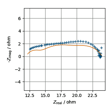
Here is a concrete example to show imcompleteness of impedance plot. Comparison of demo data bundled by pyZwx with calculated spectrum is shown by impedance plot.
The employed model and its parameter values are:
R0 + R1//CPE1 + R2//CPE2 + R3//CPE3
R0: 12
R1: 2
CPE1_T: 1e-5
CPE1_a: 0.8
R2: 6
CPE2_T: 1e-3
CPE2_a: 0.6
R3: 4
CPE3_T: 1e-2
CPE3_a: 0.7
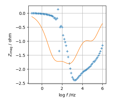
As you see, this initial guess seems to be good, but you will find this is NOT good when $\rm log \it f - Z_{\rm imag}$ is displayed.
If you start a complex nonlinear least square fit, there is a possibility to diverge the calculation.
Next, another example is shown by a spectrum measured using standard cell (SolarTron 12961).
This spectrum seems to be fit by R0 + C0 model, but you will find that estimation is incorrect when you see $\rm log (\it f \rm) - log |\it Z_{\rm imag}\rm |$ and $\rm log (\it f \rm) - log |\it Z_{\rm real}\rm |$ plots. Because you can find a "Z" like curve at $\rm log (\it f \rm) - log |\it Z_{\rm imag}\rm |$ plot around $\rm log (\it f\rm )$ = 3 to 4 region. In addition, $Z_{\rm real}$ value is not converge at fixed value at high frequency region of the $\rm log (\it f \rm) - log |\it Z_{\rm real}\rm |$ plot.
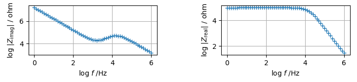
These plots indicate that R0 + C0 model is NOT appropriate for this spectrum. Although correct circuit is C0//(R1 + C1), it cannot be helped to select the model, R0//C0 + C1. Actually, it is possible to optimize the parameter using R0//C0 + C1 model.
Fitness of good is usually checked by observation that calculated curve shows good agreement with measured data. This can be purified by plots by $\rm log (\it f \rm )$ versus residuals of $Z_{\rm real}$ and $Z_{\rm imag}$. If the residuals show noisy like white noise, the model is good to reproduce the data. Oppositely, residual curves show continuos change when a model is bad for the data.
In the case of pyZwx, six graphs are displayed in one main-window. This is NOT a fashionable design but functional one to support users.
Return to the Top8. Impedance and complex permittivity
Electric amounts defined in Fourier domain are impedance, admittance, complex permittivity, and complex electric modulus. Baed on software bundling to instruments, these amounts can be translated into each other. On the other hand, it is difficult to search about the relationships among them because text displaying a conversion table is relatively easy to find by web surfine, but it would be difficult to find derived relationships among them. Here, these equations are derived from the defined equations of impedance and current.
As shown in equation (2-4), impedance and current are presented by
$Z(j\omega) = \frac{V(j\omega)}{I(j\omega)}.\ \ \ \ \ $ (8-1)
$I(j\omega) = j\omega Q(j\omega).\ \ \ \ \ $ (8-2)
Equation (8-2) can be derived from equation (2-2).
Definition of admittance is a reciprocal values of impedance, and therefore,
$Y(j\omega) = \frac{1}{Z(j\omega)} = \frac{I(j\omega)}{V(j\omega)}.\ \ \ \ \ $ (8-3)
Combined with equations (8-3) and (8-2), the following is derived.
$Y(j\omega) = \frac{j\omega Q(j\omega)}{V(j\omega)} = j\omega C_{0}\epsilon^{*}(j\omega).\ \ \ \ \ $ (8-4)
Here, complex permittivity [$\epsilon^{*}(j\omega)$)] is presented using capacitance of blank cell ($C_{0}$) by
$\frac{Q(j\omega)}{V(j \omega)} = C_{0}\epsilon^{*}(j\omega).\ \ \ \ \ $ (8-5)
From the reciprocal of equation (8-4), complex electric modulus [$M~{*}(j\omega)$] is derived.
$M^{*}(j\omega) = \frac{1}{\epsilon^{*}(j\omega)} = \frac{j\omega C_{0}}{Y(j\omega)}\ \ \ \ \ $ (8-6)
Combined with (8-6) and (8-3), the following equation is derived.
$M^{*}(j\omega) = j\omega C_{0}Z(j\omega)\ \ \ \ \ $ (8-7)
These circular relationships can be derived independent of starting equation. In addition, it is found that measurable amounts of impedance and admittance are voltage and current, but the amounts are electric charge and voltage in the case of complex permittivity and complex electric modulus. Basis of these transformation is the relation of current and electric charge.
Sometimes, we found impedance and complex permittivity are treated as different phenomena during electrochemical impedance analysis. You would understand that was a cause of mislead if you understood these relationships.
Return to the Top