Real-space observation of magnetic structures using Lorentz microscopy
Widely used imaging techniques of magnetic structures in ferromagnets include magneto-optic Faraday and Kerr microscopy, x-ray magnetic circular dichroism, magnetic force microscopy, spin polarized scanning electron microscopy, spin polarized scanning tunneling microscopy and Lorentz microscopy[1,2]. Among them, the Lorentz microscopy can provide high spatial resolution of the order of 10 nm and show high sensitivity to small changes in the local magnetization in a specimen. The method also enables investigation of relationship between the magnetic structure and the crystal structure, as it is based on transmission electron microscopy. Our group has vigorously studied magnetic structures in strongly-correlated-electron materials such as CMR manganites using low-temperature dedicated Lorentz microscopy.
The imaging is done with electrons passing through the specimen, therefore it provides essential magnetic information in the inside of specimen and low sensitivity to the local structure on the surface. However, because the magnetic structure can be affected by the shape of specimen, we must pay attention to the effect due to the thin-film shape.
[1] P. B. Hirsh et al., Electron Microscopy of Thin Crystals, p.388, Krieger (1977)
[2] T. Asaka, X. Z. Yu, K. Kimoto and Y. Matsui, J. Crystallographic Soc. Japan 47, 83 (2005).
Lorentz microscope
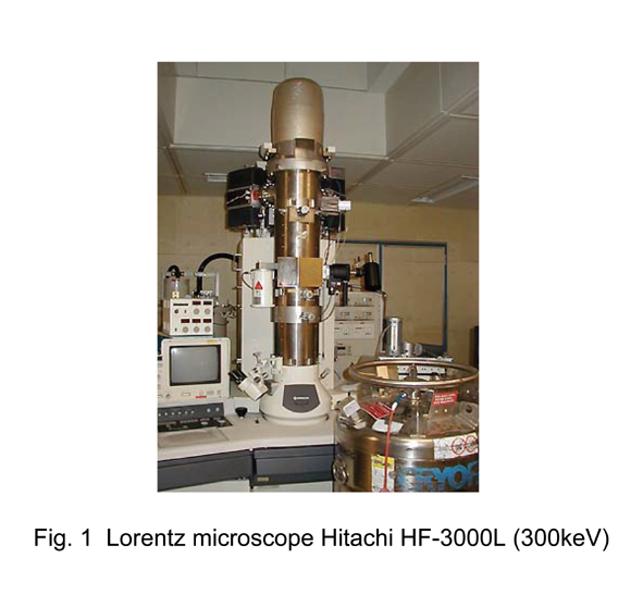
The observation is conducted with a Lorentz microscope which includes a special objective lens. We use one of the microscopes, a Hitachi HF-3000L (Fig.1) which has a field-emission electron gun with the acceleration voltage of 300keV. In usual TEM, the specimen is placed under a large magnetic field of the objective lens (~2T) that can drastically alter the magnetic structure in the specimen. The lens of Lorentz microscope gives no application of magnetic field to the specimen, which enables observation of the magnetic structure under zero field. Additionally, in order to observe response to a weak magnetic field, a field up to ~200 Oe can be applied to the specimen by an external field-generating device in our Lorentz microscope.
Fresnel method
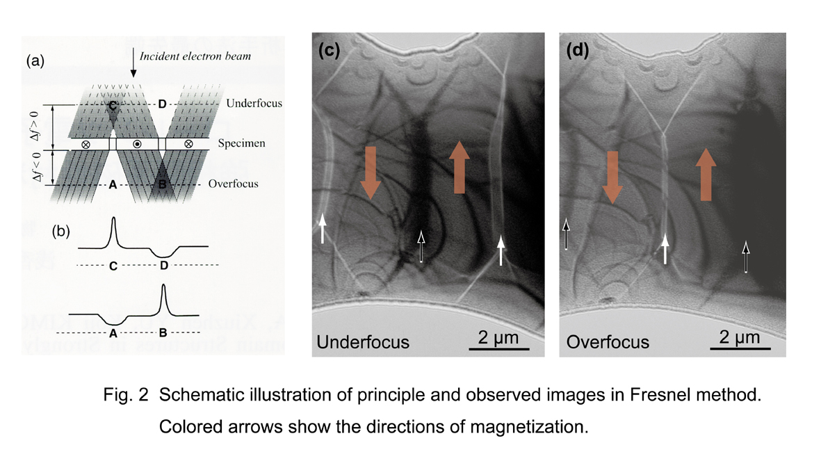
Lorentz microscopy mainly consists of two methods, Fresnel method (de-focus method) and Foucault method (in-focus method). Here, we briefly describe these imaging principles[3,4]. Figure 2(a) shows a schematic illustration of principle of Fresnel method. The specimen has 180°magnetic domain walls, which separate neighboring domains with antiparallel magnetization. Incident electron beam is deflected by Lorentz force due to the magnetization in each domain, causing variation of electron density at positions corresponding to the walls. In overfocus condition, the image plane at A-B is observed and the variation of the intensity is shown in the lower part of Fig. 2(b). By contrast, in underfocus condition, the image plane at C-D is observed and the variation of the intensity is shown in the upper part of Fig. 2(b). The low-intensity positions (A and D) and high-intensity positions (B and C) correspond to the positions of domain walls. Figures 2(c) and 2(d) display underfocused and overfocused images of ferromagnetic perovskite manganite La0.7Sr0.3MnO3 at 80K, where dark lines and bright lines that are reverse between the two images indicate the magnetic domain walls.
[3] P.J. Grundy and R. S. Tebble, Adv. in Physics 17, 153 (1968).
[4] P. B. Hirsh et al., Electron Microscopy of Thin Crystals, p.388, Krieger (1977).
Foucault method
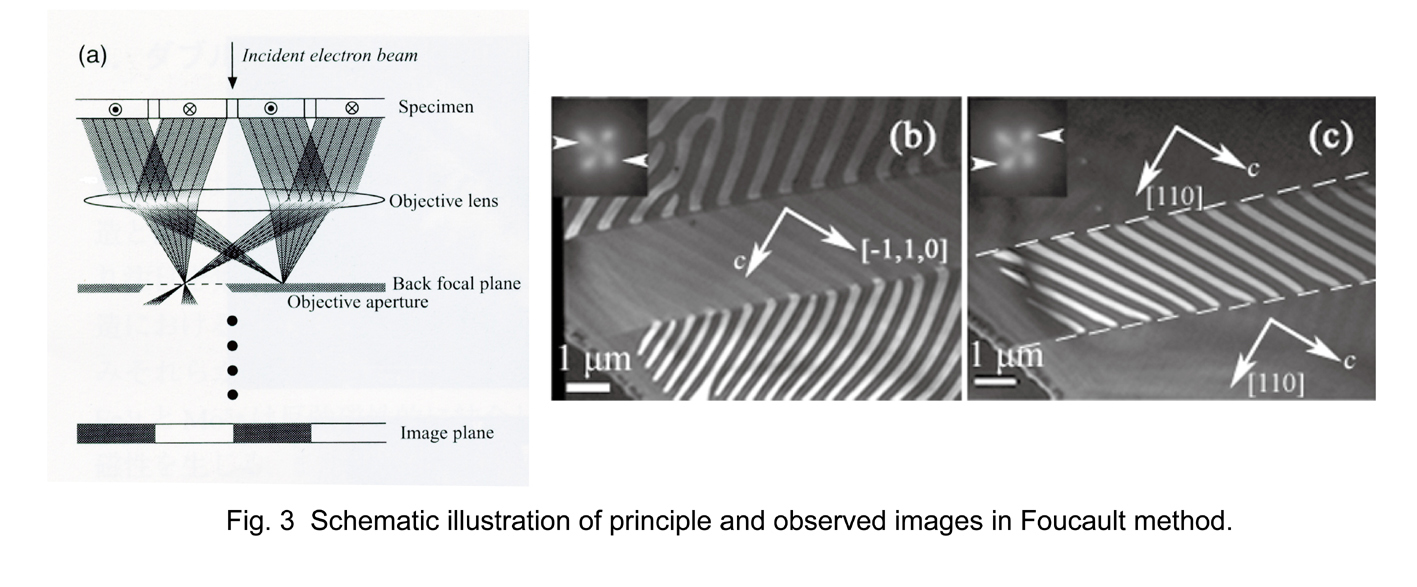
Next, a schematic illustration of principle of Foucault method is shown in Fig. 3(a). The deflected electron beam form splitted spots at the back focal plane of the objective lens. Electron beam passing through domains with the same direction of magnetization form a single spot. In Foucault method, one of the spots is selected by the objective aperture, forming an image showing the selected magnetic domains at the image plane. Figure 3(b) and 3(c) display Foucault images of La0.69Ca0.31MnO3 at ~195K [5]. The insets shows the splitted four spots indicating a perpendicular domain structure. Antiparallel domains along [110] (3(b)) and [-110] (3(c)) by selecting one of the paired spots indicated by the arrows are observed.
[5] X. Z. Yu et al.,Appl. Phys. Lett. 95, 092504 (2009).
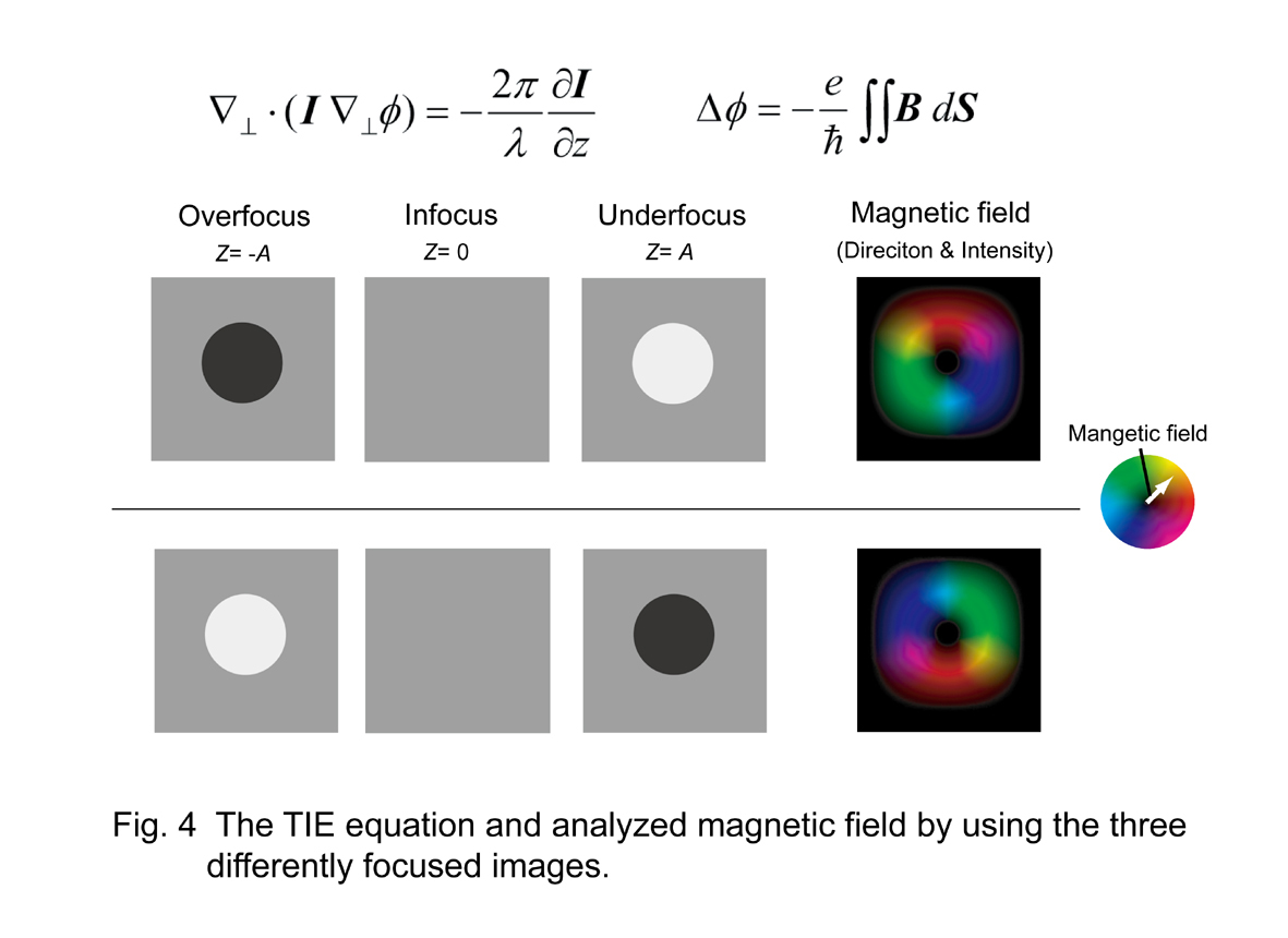
Transport-of-intensity equation technique
We use the transport-of-intensity equation (TIE) technique in order to reveal magnetization distribution in local areas. The technique was first proposed by Teague in 1983 for light optics [6], and then developed for TEM [7,8]. The TIE relates the intensity change of the electron wave along the propagation direction with the gradient of the phase in a plane perpendicular to the direction (the left equation in Fig.4). ∇is nabla operator, I the image intensity, Φ the phase of the image wave, λ the wavelength of electrons, z the defocus value. The phase can be calculated from this equation using three differently focused (in-, over-, and under-) images. The magnetic field can be obtained from the right equation. Two examples of the analysis are shown in the lower panel.
[6] M. R. Teague, J. Opt. Soc. Am. 73, 1434 (1983).
[7] D. Paganin and K. Nugent, Phys. Rev. Lett. 80, 2586 (1998).
[8] K. Ishizuka and B. Allman, J. Electron Microscopy 54(3), 191 (2005).
Magnetic structure of vortex walls in ferromagnetic nanowires
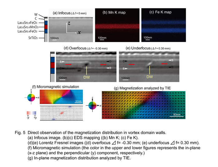
It has been reported that vortex walls, which have magnetization forming a vortex, are formed in a ferromagnetic nanowire. However, these fine spin structures have not yet been clearly observed. We successfully observed the fine structure of vortex walls using TIE technique [9]. To suppress Fresnel fringes at the edge of wire, it is necessary to enclose the ferromagnetic wire with a nonferromagnetic material, the mean inner potential of which is equivalent to that of the wire. The materials used were ferromagnetic La0.6Sr0.4MnO3 (LSMO) and antiferromagnetic La0.6Sr0.4FeO3 (LSFO). First, we fabricated an epitaxial thin-film sample in which LSFO (100 nm) / LSMO (100 nm) / LSFO (100 nm) layers were grown on a SrTiO3 substrate by pulsed-laser deposition. A cross-sectional TEM specimen was then fabricated by FIB to obtain a ferromagnetic La0.6Sr0.4MnO3 nanowire (100nm×40nm×10μm). It is hard to distinguish the LSMO wire from LSFO due to no difference in the scattering contrast in the infocus image (Fig. 5(a)), however, the LSMO wire can be clearly seen by EDS map using Mn K line (Figs. 5(b) and 5(c)). A set of Lorentz Fresnel images observed after AC demagnetization at 80 K are shown in Figs. 5(d) and 5(e). In-plane magnetization distribution given by these images, where the magnetic contrast is reversed, clearly exhibit the feature of the spin structure of vortex walls (Fig. 5(g)). The structure has twofold rotational symmetry about the center, and a Neel-wall-like area in which the magnetic moments rotate with a small radius is oriented diagonally across the wire. The anisotropic configuration is well reproduced by the micromagnetic simulation (Fig. 5(f)).
[9] T. Nagai et al., Phys. Rev. B 78, 180414 (2008)
[10] T. Nagai et al.,Materia Japan 48, 613 (2009).