Image analysis software for the scanning probe microscope
![]()
Introduction
I got an analog scanning probe microscope of high performance, NanoScope 1 sold in Japan for the first time in 1988 (at that time only the function of scanning tunnelling microscope was operated, and so images were obtained by taking photos of memory oscilloscope). Purchasing AD, DA converter and an image board, I made a digital scanning probe microscope system of high performance with machine language and Basic program language. Several years later, a really good digital scanning probe microscope, NanoScope2, was launched. It was ImageSPM that I then started to create with the effort to make it come closer to NanoScope2 in level of image display including image processing. Its performance in probe correction and automatic remove of noise with masking is superior to software on the market, with all its low performance in general.
Outline
Specialized program is added to the image analysis with scanning probe microscope based on the source cord of NIHImage1.63 in the program. It has English version of ImageSPM1.63E and 90% Japanese version of ImageSPM1.63J. The program is only for Mac. I had long been using ImageSPM1.61 made on the basis of source cord of NHIImage1.61 without opening to the public. Since the arrival of OS10 brought inconvenience in using ImageSPM, it was remade with the above-mentioned source cord, and newly opened to the public. CodeWarriorPro3 is used as a compiler. Please make sure that the author will not accept any responsibility for any problems caused during using of this program. Gold on Color Table and the function of Menu SPM are newly added. The eye-catching function is to reconstruct a image to the real image by removing most of virtual images created under the influence of the probe shape. Another function included is to remove noise by automatic wearing of mask at a specific part. This is constantly used by the author as a function of exclusively high performance.
|
1.Menu for scanning probe microscope 1.2. 3D representation of data New 1.2.1. Additional 3D display |
New 1.7.1. Slope correct between two images |
|
The data record format of scanning probe microscope depends on manufacturers. Firstly how to open the file is shown. In the data record format, the header with the record of data-obtaining information comes first, and then raw data follows in general. The size of header can be known by programs like Adobe Photoshop. For your information, the size of header is 2944 in SEIKO SP3800 often used by the author and 8192 in NanoScope3. First, select Import from file menu, and you will get the dialog shown in Fig. 1. Then, select Set in the lower right portion, and you will get the dialog shown in Fig. 2. Input the number of data of XY direction in width and height, and the size of header, in offset (others do not need to be written in). In Fig. 1, whether relocation of byte is 16 bit unsigned (SEIKO SP3800) or 16 bit signed(NanoScope3) is checked and one of them is opened. If you want to open all data at a time, Open all is checked as well. Data of the laser microscope can be saved in text data format. Leaving only the part of row data with Excel (removing header), it must be saved again. Select Import and then Text and open the file. Then it will show up on the image. |
|
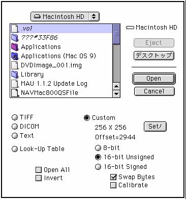
Fig. 1 |
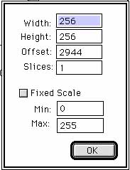
Fig. 2 |
|
1.2. 3D representation of data First two submenus, 1. 3D, 2. 3D-rotate are what display data in 3D. This part is distinctive by displaying in 3D of arbitrary tetragonal part of the image. After selecting part of the image by tetragonal selecting tool, fill in various values about the image, and even a small part can be displayed by being enlarged. Here the method to display 3D image is introduced using a text file of a laser microscope. First, select Import from a file menu. Open sample file of 3d1.txt by selecting Text in Fig. 1. Then a image shown in Fig. 3 appears. The information about the image can be found in the dialog of Info. The maximum height difference in this image is 22820nm. Select Invert from Edit menu. To correct the slope of the image, select Slope correct from SPM menu. Then select Plane correct from the dialog and input 30 for mask lebel. A flat image shown in Fig. 5 appears. After selecting part of the image with the square select tool (Fig. 5), select 3D from the sub-menu. |
|
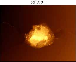
Fig. 3 |
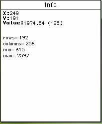
Fig. 4 |
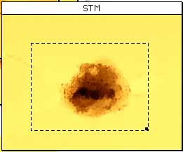
Fig. 5 |
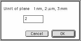
Fig. 6
Fig. 7 |
|
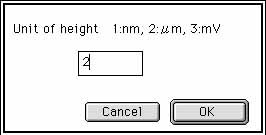
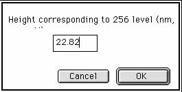
Following the program, input 2 in Fig. 7, 256 in Fig. 8, 22.82 in Fig. 9, 1 in Fig. 10, 1 in Fig. 11 and 1 in Fig. 12. 3D image shown in Fig. 13 appears. |
|
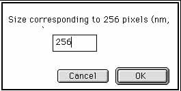
Fig. 8
Fig. 9 |
Fig. 10
Fig. 11 |
Fig. 12 |
Fig. 13 |
|
1.2.1. Additional 3D display -23/8/2005 A new 3D diplay method that any color images can be mapped on the height image will be added on imageSPM1.63cE. Fig. 51 shows the 3D image where the optical microscope image is mapped on the height image of super Kelvin force microscope. Fig. 52 shows the 3D image where the color information is mapped on the synthesized height image of color laser microscope. First, open a height image and select whole or some part of the image by the tetragonal selecting tool. Select SPM3DRGB from SPM menu. Then the dialog shown in Fig. 53 appears. Input the number of 1 for 8 bit index color image, 2 for 8 bit grey scale image or 3 for 24 bit RGB and CMYK image. In the case of 1 or 2 in number, 3D image will be made after following the indication of dialogs. In the case of 24 bit RBG image, it is necessary to prepare 8 bit R, G and B images. Photoshop can be used to create R,G and B images from 24 bit RGB image. Instead of using Photoshop, ImageJ (the author is the same person as that of NIHImage) will be used here. First, open the RBG image that will be mapped. Select RGB Split from the submenu of Color in the menu of Image. Then 8 bit R, G and B image will be made. After saving these images, open the height image and select whole or some part of the image by the tetragonal selecting tool. Select SPM3DRGB from SPM menu and input the number of 3 in the dialog shown in Fig. 53. Accoeding to the dialog, open R image and bring the 3D image to completion. Make three 3D images by using R, G and B image and save these images named as STMR, STMG and STMB respectively. Open these three images by ImageJ and select RGB Merge from the submenu of Color in the menu of Image. Then a 3D image where 24 bit RGB image is mapped will be completed. The software like Photoshop can split CMYK image, so CMYK image can be mapped by using these softwares. |
|
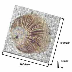
Fig. 51 |
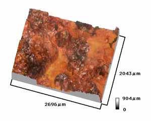
Fig. 52 |
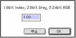
Fig. 53 |
Fig. 54 |
|
1.2.2. Change of 3D display method-23/8/2005 On ImageSPM1.63cE, four submenu for 3D display became two, that is, 3D and 3D-rotate. Rotation beween 0 and 45 degree on herizontal direction and between 0 and 90 degree on vertical direction can be done in 3D-rotate. Fig. 54 shows the 3D image with the horizontal rotation angle of 30 degree and the vertical rotation angle of 45 degree. |
|
|
The function was introduced in order to approximate the probe shape with power function by using standard sample such as grating. Open the text file of space delimiter, you will get the dialog shown in Fig. 14. It enables various curve approximations. The constant of function approximated, the standard deviation, and the coefficient of determination are shown as in Fig. 15, and can be easily obtained. The sample is provided in, please try it. |
|
Fig. 14 |
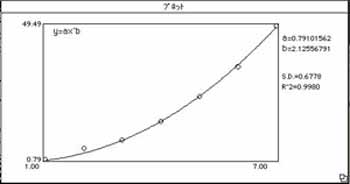
Fig. 15 |
|
This is the preeminent of this program. This program was made when the author was in the headquarters about ten years ago. The correction of program in this time enables to show the progeress of the procedure by 1 % step. You can also exit the loop by pressing Command + Period. When images are obtained by scanning probe microscope, the side face of the probe, not its tip, touches on the sample with the shape of large irregularity. For instance, the step shown in Fig. 16 is scanned, the shape then obtained becomes what is shown in bold solid line. The principle of image reconstruction is: set a virtual probe up on an image, and the part shown by oblique lines in Fig.16 is overlapped. By removing the overlapped part, an image close to the real is reconstructed. At present this is the most accurate correction technique considered. In order to explain why the further correction is not possible, the shape without the overlapped part (shown as the curved thin solid line) is considered. Scanning this shape produces the shape shown with the bold solid line, equivalent to that obtained by scanning the step. Namely, to obtain the equivalent shape to that with scanning the step shows the limit of correction. Then how can we get better images? My suggestion is: given the scanning shape left to right, when the height is considered to increase, the probe is inclined anticlockwise by several degrees. On the contrary, when the height decreases, it is inclined clockwise by several degrees. |
|
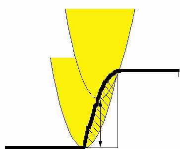
Fig. 16 |
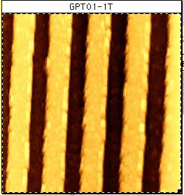
Fig. 17 |
|
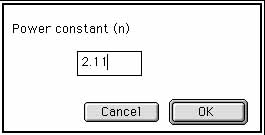
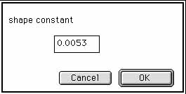
Back to the main theme, two kinds of image correction method are provided. One is the method that the probe shape is approximated with a function, where the power function is adopted in the program. The other is one with the probe image, considering the probe shape difficult to be approximated with a function. The sample image of grating in Fig. 17 was taken 10 years ago, where the probe shape had 2.11 of power constant and 0.0053 of shape constant. The late brand new probe had 1.71 of power constant and 0.0498 of shape constant. It will be found out that with the use of these values, reconstructing images leads to almost the real one. The process is explained in detail. First open the sample image GPT01-1T. Select the part of image reconstruction (The full figure is selected in Fig. 17.). Then select SPM deconvolution f from sub-menu. After that enter the scanning area in Fig. 18, the power constant in Fig. 19, the height and width of the image in Fig. 20, and the shape constant in Fig. 21, then the image reconstruction will start. The process is shown in the dialog information at the lower left as shown in Fig. 22. In the case that it takes too long, exit the program with pressing command + period. When the image reconstruction finishes, it will be found out that the image as shown in Fig. 23 is constructed. |
|
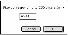
Fig. 18
Fig. 19 |
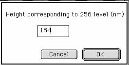
Fig. 20
Fig. 21 |
Fig. 22 |
Fig. 23 |
|
Next, on the contrary, let's try SPM simulation. The process is all the same. It will be found out that the image close to one in Fig. 17 is constructed. The simulation and the image reconstruction with a probe image are also introduced. This program was made because I wanted to know how images are influenced in the triangular pyramid probe used in nanoindentation and the nanotube probe . If the probe shape is known with SEM, this can be used making the image. As for how to see probe images, for instance, the tip becomes the triangular pyramid and the other part, the triangle pole, in the triangular pyramid probe. Now the actual usage is shown. This is the image simulation in the case that the tip of the probe gets cracked, called the double tip effect. First the image of STM is opened. After selecting all, select SPM simulation image from the sub-menu of SPM, and you will first get the same dialog as Fig. 18. Input the size of the real image of 2000. Next, since you get the same as Fig. 20, input 18. Then, since you get the alert saying to select the probe image, click ok, and open sprobe3 here. Since you get the dialog same as Fig. 18, input 1000 here (500 is also ok). After that, since you get the dialog same as Fig. 20, input 20. Now the image simulation starts. When it finishes, the image in Fig. 24 is constructed (note: the image processing cannot be done in the part half as wide as the probe of the marginal area). Fig. 25 is the image taken with the probe considered as the double tips. It is characterized by the appearance of similar patterns in the image. In the case that these images appear, it is important to change the probe and take images once again. |
|
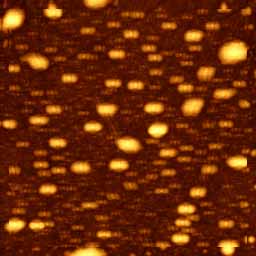
Fig. 24 |
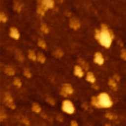
Fig. 25 |
|
Next, let's try the image reconstruction with the use of the same probe image. The process is the same as in the case of simulation. The image like Fig. 26 will be constructed. It will be found out that even the use of such a probe can approximate to the original image. It may be a fun to try all kinds. |
|
Fig. 26 |
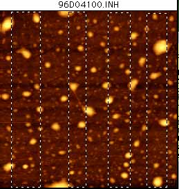
Fig. 27 |
|
This is the second distinctive of this program. In the case that the image of small droplet existing on the very flat plane like graphite is taken, the nonexistent difference of elevation appears as noise by temperature drift. The usage in that case is explained. First, open the sample image 96D04100.INH. Select all (note: The specific part can be selected as in Fig. 27. In the case that several parts are selected, select during pressing the control key. In this case the noise removal with the consideration of the area selected is executed), and select Correct slope from the submenu of menu SPM. Then you will get the dialog like Fig. 28. The first four is a kind of the function of flat. The author uses the first two a lot. Select Vertical linear correct, the second one, here. Then, the dialog in Fig. 29 is shown. Where with the input of 30, the image without noise is constructed. The smaller the value of mask lebel is, the finer the removed noise is. In the case that there is a large swell, the assignment of a large numerical value is needed. Try all kinds and seek the most suited condition. |
|
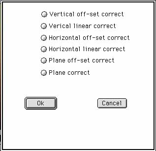
Fig. 28 |
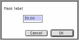
Fig. 29
Fig. 30 |
|
1.5.1. Additional function for slope correct 1 - 29/6/2005 A lot of functions for slope correct will be added on ImageSPM1.63aE. First, Plane quadratic correct will be added on the dialog shown in Fig. 28. Mask area will be able to select as shown in Fig. 43. Mask will not operate on 1.Off. Mask lebel of both upper and lower part can be set on 2. Both. Mask lebel of upper (bright) part ca be set on 3. Up (Fig. 45). Mask lebel of lower (dark) part can be set on 4. Low. Level correct will be able to do as shown in Fig. 44. To input a positive value makes the image darker (lower). As for Plane correct, the slope correct will be able to do using the information of the selected area by selecting the square selection tool. This function causes the enoumous change of height scale, so the function to fit the height scale automatically will be added (Fig. 46). When the automatic scaling function is operating, the ratio of magnified height is indicated on the Info dialog like 1017%. It is necessary to input the height value of 10.17 times as former one when 3D image display is selected. The interesting thing to use this function is that the image shown in Fig. 47 can be displayed as the image shown in Fig. 48. Plane quadratic correct can also do the slope correct using the imformation of selected area. However, the automatic scaling function can not work at the moment. Hereafter the mask function will be explained by using the sample image of 96D04100.INH. After the image is opened, execute sub-menu of Measure from menu of Analyze. Then Mean in Info dialog shows the value of 204.18. This value is the mean density of this image. When the value of 30 is inputted in Mask lebel up as shown in Fig. 45, the density area lower than 174.18 which is derived from the calcuration of 204.18 -30 will be masked (not considered in the calcuration ). On the other hand, the density area higher than 234.18 will be masked in the case of Mask lebel low. Thus the mask lebel can be estimated by using the wand tool. |
|
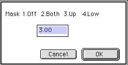
Fig. 43 |
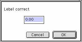
Fig. 44 |
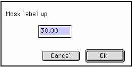
Fig. 45 |

Fig. 46 |
Fig. 47 |
Fig. 48 |
|
1.5.2. Additional function for slope correct 2 - 13/7/2005 The automatic scaling function will be added on menu of Slope correct on ImageSPM1.63bE. In addtion, Menu of Manual will be added on the dialog of Auto scaling as shown in Fig. 49. Dialog of magnification (Fig. 50) will appear when Manual is selected, so input the magnification. |
|
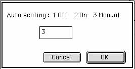
Fig. 49 |
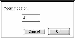
Fig. 50 |
|
This is the same function as the line edit, where the data around is simply set in the noise area. After the noise area is selected, select scratch correction from the submenu. Then it is excuted. |
|
|
Since the author seldom uses them, they are not explained. They were made just for fun. |
|
|
1.7.1. Slope correct between two images - 2/8/2005 The function that the slope becomes the same between selcted two images will be added on ImageSPM1.63cE. The purpose of adding this function is to unify the color lebel for the height at movie making. This function is also useful for the accurate image subtraction. First, open the base image. Then select SPMsub from sub-menu of menu of SPM. Input the value of height corresponding to the 256 lebel. After this, a dialog that ask you to choose the image to be corrected will appear. Choose the image and follow as the dialog indicates. |
|
|
Estimatation can be done using samples such as grating and square pole. When scanning is done on the step shape shown in Fig. 6, the upside-down image of probe is produced at the edge of the step. Save the profile of cross section as a text file and make approximation of pobe shape by power function. This is the case of approximation by function. As for image approximation, the image shown in Fig. 31(b) is obtained when a square pole shown in Fig. 31(a) is scanned. The upside-down pobe image can be obtained from the image of 4 corners. |
|
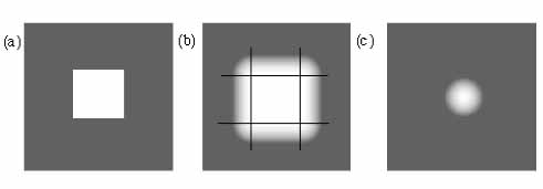
Fig. 31 |
|
|
When we take an image by an optical microscope, uneven color often appears especially if the contrast is increased as shown in Fig. 32. This uneven color can be corrected easily by using a special image treatment (Fig. 33). The method will be shown after the procedure to get a patent. |
|
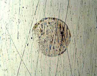
Fig. 32 |
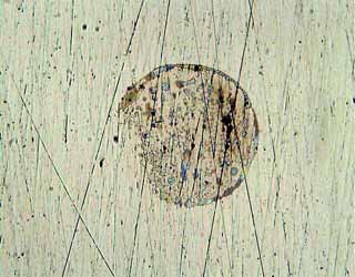
Fig. 33 |